Input files for MLPF use a syntax similar to MCTDH. Parameters are organized into sections, which are enclosed in directives like
XXX-SECTION
END-XXX-SECTION
The file must end with the directive END-INPUT.
The following describes the individual sections.
This section controls parameters for input, output, and what exactly to compute. Directives are simply keywords, or of the form keyword = parameter(s). The following table lists the available directives. S specifies a string, I an integer, and R a real-valued parameter, which might include a unit (in the same manner as MCTDH, e.g. "1.0,eV"). Square brackets indicate optional parameters.
| Directive | Description |
|---|---|
| name = S | Output will be put into the directory S. |
| gendvr | DVR information will be generated and stored it in the file dvr. This requires a PRIMITIVE-BASIS-SECTION to be present |
| readdvr [= S] | DVR information will be read from the file S. If unspecified, S is dvr. |
| genpot | A full-grid potential will be computed and stored, in a format depending on vpot-format. (not yet implemented) |
| readvpot [= S] | A full-grid potential will be read from the file S. If unspecified, S is vpot or vpot2, depending on vpot-format. |
| readnpot [= S] | A Potfit potential will be read from the file S. If unspecified, S is natpot. |
| vpot-format = I | Format for full-grid potential. I must be 1 or 2. |
| rmse = R | Set the maximum allowed root-mean-square error of the fitted potential to R. |
| graphviz | Produce a file tree.dot which can be used to visualize the multi-layer tree using Graphviz. |
(may be abbreviated to PBASIS-SECTION)
This section defines the coordinate system, and which grid points to use for each coordinate. Each line describes one primitive coordinate, using the syntax
Modelabel BasisType Parameters...This is the same format as the corresponding section in MCTDH. Therefore, please see the corresponding MCTDH documentation for details of specifying the basis and parameters.
The idea is that you can copy & paste your PBASIS-SECTION from your MCTDH input file. However, there are currently two caveats:
This section defines how the primitive modes are hierarchically combined into larger and larger modes, and (optionally) specifies how many "single-particle potentials" (SPPs) should be used for each mode. So this section fulfills a similar role to the ML-BASIS-SECTION used in MCTDH for ML-MCTDH runs, but the syntax is rather different. Instead, the syntax in the TREE-SECTION is a minimal extension of the syntax used in the NATPOT-BASIS-SECTION in Potfit and the SPF-BASIS-SECTION in MCTDH input files.
The basic element in this section is a statement of the form
Modelabel1 [, Modelabel2 ... ] [ = nspp ]which signifies that the given modelabels (which must have been present in the PBASIS-SECTION) are combined into a primitive mode, and that nspp SPPs should be employed for this mode. To combine the primitive modes into higher-layer modes, simply group the primitive modes together with parentheses. After the closing parenthesis, you can (optionally) specify the number of SPPs for the combined mode, again using = nspp. This mode grouping must be applied recursively, such that you eventually enclose the whole block by one final pair of parentheses.
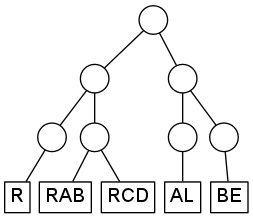
To give an example, suppose that your system contains five degrees of freedom, with modelabels R, RAB, RCD, AL, and BE. You want to organize the modes into the following hierarchy:
Without specifying the number of SPPs, the corresponding TREE-SECTION is:
TREE-SECTION
(
  (
    R
    RAB,RCD
  )
  (
    AL
    BE
  )
)
END-TREE-SECTION
Line-breaks are not significant here, so you might as well write:
TREE-SECTION
( ( R  RAB,RCD )  ( AL BE ) )
END-TREE-SECTIONMost likely not. What you usually want is a potential fit which fulfills a certain accuracy criterium. MLPF supports this by setting the allowed global root-mean-square error of the fit with the rmse parameter in the RUN-SECTION. If this is supplied, and no SPP numbers are given in the TREE-SECTION, then the following strategy is applied:
If the TREE-SECTION specifies the number of SPPs for any mode, then that number is used, instead of the one which the above algorithm would choose. If the number of SPPs is only specified for some but not all modes, then the situation may arise that the RMSE budget is exhausted before the top is reached. In this case MLPF will produce a fit which is not truncated in the higher layers, which is far from optimal. Hence, if you specify the number of SPPs for any mode, you should do so for all modes, and live with whatever RMSE results from that.
The (estimated) RMSE error for each mode, and the number of SPPs chosen, is written to the log file.